SELFE v2.0ha User Manual
Input files
Horizontal grid (hgrid.gr3):
In xmgredit grid format.
Below is a sample:
fort_12062002.14 : alphanumeric description
55880 30001 : # of elements and nodes in the horizontal grid
(Coordinate
part):
1 386380.409604 286208.187634 5.122
: node #, x,y, depth
2 386460.352736 285995.038877 9.167
3 386687.720000 286213.590000 1.000
4 386460.076848 286367.779818 2.209
5 386678.380000 286483.440000 1.614
6 386180.219063 286405.956765 4.627
7 386409.007263 286563.660632 2.629
8 386186.575437 286680.225393 4.195
9 385958.392423 286604.196847 4.177
.............................................
(Connectivity part)
2 3 3 4 5
3 3 3 5 6
4 3 1 4 6
5 3 4 7 9
...........................................
(Boundary condition part)
3 : Number of open boundaries
95 : Total number of open boundary nodes
85 : Number of nodes for open boundary 1
15185 : first node
........................................
25 = number of land boundaries
4079 = Total number of land boundary nodes
1452 0 = Number of nodes for land boundary 1
19947 : first node
19945
19943
.......................................
Note: (1) the boundary condition (b.c.) part can be generated with xmgredit5 --> GridDEM --> Create open/land boundaries;
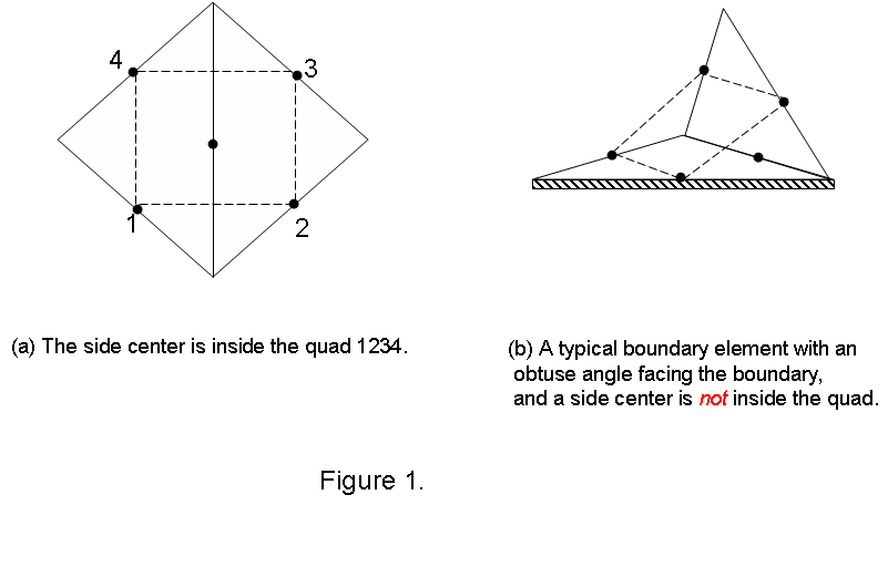
(2) The use of a Shapiro filter (indvel=0 or -1) places some constraints on the boundary sides. In particular, the center of any internal sides must be inside the quad formed by the centers of its 4 adjacent sides (see Fig. 1). If not, the code will try to enlarge the stencil, but if the side is near the boundary, fatal error will occur. To find out all violating boundary elements, just prepare hgrid.gr3 (note that the open boundary info needs no be correct at this stage), vgrid.in and param.in up to ihorcon, and run the code with ipre=1 in param.in. You'll find a list of all such sides in fort.11 (the two node numbers of a side will be shown). Method to eliminate this problem includes: (1) move node, (2) swap the side for a pair of elements, and (3) refine or coarsen. Note that in most grid editors, the first 2 methods won't change the node numbering and so you'd try them first before Method (3), to save time. After the pre-processing run is successful (with a screen message indicating so), you can then proceed to prepare other inputs.
Vertical grid (vgrid.in)
This version uses hybrid S-Z coordinates in the vertical, with S on top of Z.
54 18 100. !nvrt; kz (# of Z-levels); h_s (transition depth between S and Z)
Z levels !Z-levels first
1 -5000. !level index, z-coordinates
2 -2300.
3 -1800.
4 -1400.
5 -1000.
6 -770.
7 -570.
8 -470.
9 -390.
10 -340.
11 -290.
12 -240.
13 -190.
14 -140.
15 -120.
16 -110.
17 -105.
18 -100. !
S levels !S-levels below
30. 0.7 10. ! constants used in S-coordinates: h_c, theta_b, theta_f (see notes
below)
18 -1. !first S-level (S-coordinate must be -1)
19 -0.972222 !levels index,
20 -0.944444
.......
54 0. !last
Notes:
Boundary conditions and tidal info (bctides.in)
48-character
start time info string, e.g., 04/23/2002 00:00:00 PST (only used for
visualization with xmvis)
ntip, tip_dp: # of constituents used in earth tidal potential;
cut-off depth for applying
tidal
potential (i.e., it is not calculated when depth <
tip_dp).
For k=1, ntip
talpha(k) = tidal constituent name;
jspc(k), tamp(k), tfreq(k), tnf(k), tear(k) = tidal species # (0: declinational; 1: diurnal; 2: semi-diurnal), amplitude constants, frequency, nodal factor, earth equilibrium argument (in degrees);
end for;
nbfr
= total # of tidal boundary forcing frequencies.
For
k=1, nbfr
alpha(k)
= tidal constituent name;
amig(k), ff(k), face(k) = forcing frequency,
nodal factor, earth equilibrium argument (in degrees) for constituents
forced on the open boundary;
end
for;
nope: # of open boundary segments;
For
j=1, nope
neta(j), iettype(j), ifltype(j), itetype(j), isatype(j) = # of nodes on the open boundary segment j (from hgrid.gr3), b.c. flags for elevation, normal velocity, temperature, and salinity;
if (iettype(j) == 1) !time history of elevation on this boundary
no input in this file; time history of elevation is read in from elev.th;
else if (iettype(j) == 2) !this boundary is forced by a constant elevation
ethconst: constant elevation
else if (iettype(j) == 3) !this boundary is forced by tides
for k=1, nbfr
alpha(k) = tidal constituent name;
for i=1, neta(j)
emo(ietaelem(j,i),k), efa(ietaelem(j,i),k) !amplitude and phase for
each node on this open boundary;
end for
end for;
else
elevations are not specified for this boundary (in this case the velocity must be specified).
endif
if (ifltype(j) == 0) !nornal vel. not specified
no input needed
else if (ifltype(j) == 1) !time history of discharge on this boundary
no input in this file; time history of discharge is read in from flux.th;
else if (ifltype(j) == 2) !this boundary is forced by a constant discharge
vthconst: constant discharge (note that a negative number means inflow)
else if (ifltype(j) == 3) !vel. is forced in frequency domain
for k=1, nbfr
vmo(j,k),vfa(j,k) !uniform amplitude and phase along each boundary segment
end for;
eta_m0,qthcon(j): mean elevation and discharge on the jth boundary
endif
if (itetype(j) == 0) !temperature not specified
no input needed
else if (itetype(j) == 1) !time history of temperature on this boundary
no input in this file; time history of temperature is read in from temp.th;
else if (itetype(j) == 2) !this boundary is forced by a constant temperature
tthconst = constant temperature
else if (itetype(j) == 3) !keep initial temperature profile
no input is needed
else if(itetype(j) == -1) !open b.c.; nudge to initial condition
tobc: nudging factor (between 0 and 1).
else if(itetype(j) == -4) ! nudge to 3D time series in temp3D.th
tobc: nudging factor (between 0 and 1).
endif
Salintiy
b.c. is similar to temperature:
if (isatype(j) == 0) !salinity not specified
.........
endif
This file uses free format, i.e. the order of each input parameter is not important. Governing rules for this file are:
ipre:
pre-processing flag. ipre=1:
code will output centers.bp, sidecenters.bp, obe.out (centers build point,
sidcenters build point, and list of open boundary elements), and
mirror.out and stop. This
is useful also for checking geometry violation, z-levels at various depths (in mirror.out) for any given
choice of vgrid. IMPORTANT: ipre=1 only works for single CPU! ipre=0:
normal run.
ntracers
: total number of passive tracers.
imm: tsunami option. Default: 0 (no bed deformation); 1: with bed deformation (needs bdef.gr3).
If imm=1, this
line is ibdef: total # of deformation steps (i.e., the bed will
change from the initial position to the position specified in bdef.gr3 in
ibdef steps).
ihot
= hot start flag. If ihot=0, cold start; if ihot/=0, hot start from
hotstart.in. If ihot=1, the time and time step are reset to
zero, and outputs start from t=0 accordingly. If ihot=2, the run (and output) will continue from the time specified in
hotstart.in.
ics
= coordinate frame flag. If ics=1, Cartesian coordinates are
used; if ics=2, degrees latitude/longitude are used (but the output
will still be in
Cartesian coordinates).
cpp_lon,
cpp_lat= centers of projection used to convert lat/long to Cartesian
coordinates. These are used for ics=2, or a variable Coriolis parameter
is employed (ncor=1), or the heat exchange sub-model is invoked (ihconsv=1).
ihorcon: flag to
use non-zero horizontal viscosity. If
ihdif: flag to
use non-zero horizontal duffusivity. If
thetai
= implicitness parameter (between 0.5 and 1). Recommended value: 0.6.
ibcc,
itransport= barotropic/baroclinic flags. If ibcc=0, a baroclinic model is used
and regardless of the value for itransport, the transport equation is solved. If
ibcc=1, a barotropic model is used, and the transport equation may (when
itransport=1) or may not (when itransport=0) be solved; in the former case, S and T are
treated as passive tracers.
If
ibcc=0, the ramp-up fucntion is specified as:
rnday
= total run time in days.
nramp,
dramp = ramp option for the tides and some boundary conditions, and ramp-up
period in days (not used if nramp=0).
dt
= time step (in sec).
h0
= minimum depth (in m) for wetting and drying (recommended value: 1cm). When the total depth is less than h0, the
corresponding nodes/sides/elements are considered dry. It should always be
positive to prevent underflow.
bfric
= bottom friction option. If bfric=0, spatially varying drag coefficients are
read in from drag.gr3 (as depth info). For bfric=1, bottom roughnesses (in
meters) are read in from rough.gr3.
If
bfric=1, maximum drag coefficient is specified as Cdmax (to prevent
exaggeration of drag coefficient in shallow areas).
ncor
= Coriolis option. If ncor=0 or -1, a constant Coriolis parameter is used
(see next line). If ncor=1,
a variable Coriolis parameter, based on a beta-plane approximation, is used,
with the lat/long. coordinates read in from
hgrid.ll.
In this case, the center of CPP projection must be correctly specified (see
above).
If
ncor=0, 'coriolis' = constant Coriolis parameter.
nws,
wtiminc = wind forcing options and the interval (in seconds) with which the
wind input is read in. If nws=0, no wind is applied (and wtiminc becomes
immaterial). If nws=1, constant wind is applied to the whole domain at any
given time, and the time history of wind is input from
wind.th. If
nws=2 or 3,
spatially and temporally variable wind is applied and the input consists of a number of
netcdf
files in the directory sflux/.
If
nws>0, the ramp-up option is specified as: nrampwind, drampwind = ramp option and period
(in days) for wind.
ihconsv,
isconsv = heat budget and salt conservation models flags. If ihconsv=0, the heat budget model is not used. If
ihconsv=1, a heat budget model is invoked, and a number of
netcdf files for radiation flux
input are read in from he directory sflux/.
itur
= turbulence closure model selection. If itur=0, constant diffusivities are
used for momentum and transport (and the values are specified in the next
line). If itur=-2, vertically homogeneous but horizontally varying
diffusivities are used, which are read in from
hvd.mom.and
hvd.tran.
If
itur=0, the constant viscosity and diffusivity are: dfv0, dfh0.
If itur=2, the next line is: h1_pp, vdmax_pp1, vdmin_pp1, tdmin_pp1, h2_pp, vdmax_pp2, vdmin_pp2,tdmin_pp2. Eddy viscosity is computed as: vdiff=vdiff_max/(1+rich)^2+vdiff_min, and diffusivity tdiff=vdiff_max/(1+rich)^2+tdiff_min, where rich is a Richardson number. The limits (vdiff_max, vdiff_min and tdiff_min) vary linearly with depth between depths h1_pp and h2_pp.
If itur=3, the next line is:
turb_met, turb_stab: choice of model description ("MY"-Mellor & Yamada, "KL"-GLS as k-kl, "KE"-GLS as k-epsilon, "KW"-GLS as k-omega, or "UB"-Umlauf & Burchard's optimal), and stability function ("GA"-Galperin's, or "KC"-Kantha & Clayson's for GLS models). In this case, the minimum and maximum viscosity/diffusivity are specified in diffmin.gr3 and diffmax.gr3, and the scale for surface mixing length is specified in xlfs.gr3.
If itur=4, GOTM turbulence model is invoked; the user needs
to compile the GOTM libraries first (see FAQ or README inside GOTM/ for
instructions), and turn on
icst = options for specifying initial temperature and salinity field
for cold start. If icst=1, a vertically homogeneous but horizontally
varying initial temperature and salinity field is contained in
temp.ic and
salt.ic. If
icst=2, a horizontally
homogeneous but vertically varying initial temperature and salinity
field, prescribed in a series of z-levels, is contained in
ts.ic.
ibcc_mean: mean T,S profile option. If ibcc_mean=1 (or ihot=0 and icst=2), mean profile
is read in from ts.ic, and will be removed when calculating baroclinic force.
No ts.ic is needed if ibcc_mean=0.
iwrite: output format option; not active and
probably will be removed eventually.
nspool,
ihfskip: Global output skips. Output is done every nspool steps, and
a new output stack is opened every ihfskip steps.
Therefore the outputs are named as [1,2,3,...]_[process id]_salt.63 etc.
next
25+ lines are global output (in machine-dependent binary) options. The (process-specific)
outputs share similar
structure. Only the first line is detailed here.
elev.61 = global
elevation output
control. If
'elev.61' =0, no global elevation is recorded. If 'elev.61'=
1, global elevation for each
node in the grid is recorded in [1,2,3...]_[process id]_elev.61 in binary format.
The
output is either starting from scratch or appended to existing ones
depending on ihot.
pres.61: output options for atmospheric pressure (*pres.61). airt.61: output
options for air temperature (*airt.61). shum.61: output
options for specific humidity (*shum.61). srad.61: output
options for solar radiation (*srad.61). flsu.61: output
options for short wave radiation (*flsu.61). fllu.61: output
options for long wave radiation (*fllu.61). radu.61: output
options for upward heat flux (*radu.61). radd.61: output
options for downward flux (*radd.61). flux.61: output
options for total flux (*flux.61). prcp.61:
output options for precipitation rate (*prcp.61). wind.62: output
options for wind speed (*wind.62). wist.62: output
options for wind stresses (*wist.62).
vert.63: output
options for vertical velocity (*vert.63). temp.63: output
options for temperature (*temp.63). salt.63: output
options for salinity (*salt.63). conc.63: output
options for density (*conc.63). tdff.63: output
options for eddy diffusivity (*tdff.63). vdff.63: output
options for eddy viscosity (*vdff.63). kine.63: output
options for turbulent kinetic energy (*kine.63). mixl.63: output
options for macroscale mixing length (*mixl.63). zcor.63: output
options for z coordinates at each node (*zcor.63).
hvel.64: output
options for horizontal velocity (*hvel.64).
hotout,hotout_write = hot start output control parameters. If hotout=0, no hot
start output is generated. If hotout=1, hot start output is spooled to it_[process id]_hotstart every
hotout_write
time steps, where
it is the
corresponding time iteration number, and hotout must be a multiple of ihfskip above. If a run needs to be hot started from step
it, the user needs to combine all process-specific hotstart outputs into a hotstart.in
using combine_hotstart*.f90.
slvr_output_spool,mxitn,tolerance
= parallel JCG solver control parameters. Recommended
values: 50 1000 1.e-12.
consv_check = parameter for checking
volume and salt conservation. If
turned on (=1), the conservation will be checked in regions specified by
fluxflag.gr3.
inter_st,
inter_mom: linear (inter_st=1) or quadratic (inter_st=2) interpolation for T, S in backtracking,
and linear (
depth_zsigma:
Option for computing baroclinic force near bottom. If the local depth
is less than depth_zsigma, constant extrapolation is used; otherwise
a more conservative approach is used to minimze inconsistency.
inu_st,
step_nu, vnh1,vnf1,vnh2,vnf2: nudging flag for S,T, nudging step,
parameters for vertical nudging. When inu_st=0, no nudging is done. When
inu_st=1, nudge to initial conditions. When inu_st=2, nudge to values
specified in temp_nu.in and salt_nu.in, given at an interval of
step_nu.
For inu_st/=0, the horizontal nudging factors are
given
in t_nudge.gr3 and s_nudge.gr3 (as depths info), and the vertical nudging factors vary
linearly along the depth as: min(vnf2,max(vnf1,vnf)),
where vnf=vnf1+(vnf2-vnf1)*(h-vnh1)/(vnh2-vnh1).
The nudging factor is the sum of the two. idrag: bottom drag option. idrag=1: linear drag formulation; idrag=2:
quadratic drag
ihhat: wet/dry option. If ihhat=1, the friction-reduced depth will be kept
non-negative to ensure robustness (at the expense of accuracy); if ihhat=0,
the depth is unrestricted.
iupwind_t: upwind option for T,S. A value of "0"
corresponds to Eulerian-Lagrangian transport option (and the interpolation
method is determined by inter_st above), "1" for the
mass-conservative upwind option, and "2" for the higher-order
blend_internal,
rmaxvel: maximum velocity. This is needed mainly for the air-water exchange
as the model may blow up if the water velocity is above 20m^2/s.
velmin_btrack: minimum velocity before backtracking is invoked. e.g., 1.e-3 (m/s).
If ntracers>0,
additional lines are needed that specify the transport method (upwind or TVD)
and horizontal boundary conditions etc. Consult the source code for details.
See FAQ for how to interface your own code to SELFE.
Depending on the values of icst (see parameter input file):
Bottom drag (drag.gr3 or rough.gr3)
grid !file decription
40000
27918 !# of elements, # of nodes
1 386738.500000 285939.060000 0.004500 !node #, x, y, drag coefficient Cd (for
nchi=0) or roughness (in meters; for nchi=1)
2 386687.720000 286213.590000 0.004500
3 386421.090000 286172.160000 0.004500
4 386471.720000 286376.030000 0.004500
5 386678.380000 286483.440000 0.004500
6 386140.190000 286439.220000 0.004500
7 386387.280000 286557.310000 0.004500
8 386209.840000 286676.470000 0.004500
..........
If nws=1 in param.in, a time history of wind speed must be specified in this file:
5. 8.660254 ! x and y components of wind speed @ 0*wtiminc
5. 8.660254
5. 8.660254
.......
Note that the speed varies linearly in time, and the time interval (wtiminc) is specified in param.in.
This includes elev.th, flux.th, temp.th, salt.th, which share same structure. Below is a sample flux.th:
300. -1613.05005 -6186.60156 !time (in sec), discharge at the 1st boundary
with ifltype=1, discharge at the 2nd boundary with ifltype=1
600. -1611.37854 -6208.62549
900. -1609.39612 -6232.22314
1200. -1607.42651 -6254.24707
1500. -1605.45703 -6276.27148
1800. -1603.48743 -6298.2959
2100. -1601.3772 -6321.89307
2400. -1599.40772 -6343.91748
2700. -1597.43811 -6365.94141
3000. -1595.46863 -6387.96582
3300. -1593.49902 -6409.99023
3600. -1591.38879 -6433.5874
3900. -1589.41931 -6452.94287
4200. -1587.2959 -6472.29834
...........
Space- and time-varying time history inputs (*3D.th):
These include elev3D.th, uv3D.th, temp3D.th, salt3D.th, which share similar binary structure. For example, uv3D.th:
for it=1,nt !all time steps
read(12,rec=it)time,((uth(k,i),vth(k,i),k=1,nvrt),i=1,nodes); !all open-boundary nodes that need this type of b.c.
end for !it
This file is generated with the pre-processing flag in param.in for debugging purpose only.
3 # of open bnd
Element list:
251 bnd # 1
1 31587
2 31588
3 31589
4 31590
5 31592
6 31595
7 31601
8 31603
9 31605
10 31606
........
4 bnd # 2
1 31583
2 31584
3 31585
4 31586
........
If nadv=0, the advection on/off flags are the "depths" (0: off; 1: Euler; 2: 5th order Runge-Kutta) in this grid file, which is otherwise similar to hgrid.gr3.
The depth specifies the Kriging option for each node: 0 means no Kriging; 1 means applying Kriging there. The order of the generalized covariance function is specified
in param.in.
The depth specifies the minimum and maximum diffusivity imposed at each node. This is needed to further constraint outputs from the GLS model. We generally recommend a constant value of 1.e-6 m^2/s for minimum diffusivity, and 1.e-2 m^2/s for maximum diffusivity inside estuaries and 10 m^2/s otherwise. The minimum diffusivity may also be changed locally, e.g., to create a mixing pool near the end of a river.
The depth specifies the surface mixing length used in GLS model in meters. We recommend using a constant value equal to the maximum surface layer thickness in the domain, but the users
may try smaller values as well.
The depth specifies the way the vertical interpolation is done locally, i.e., along Z or S plane. If the depth=1, it is done along Z-plane; if the depth=2, along S-plane. We recommend the value of 2 in "pure S" zone, and 1 in SZ zone. You may not use "2" in the SZ zone.
Lat/long coordinates (hgrid.ll)
This file is identical to hgrid.gr3 except the x,y coordinates are replaced by lattitudes and longitudes.
This consists of a suite of input for wind and radiation fluxes found in a sub-directory sflux/. When nws=2, the wind speed and atmospheric pressure are read in from this directory; when ihconsv=1, various fluxes are read in from it as well. The netcdf files for various periods have been pre-computed by Mike Zulauf and deposited in a data base.
Conservation check files (fluxflag.gr3)
vvd.dat, hvd.mom, and hvd.tran
Amplitudes and phases of boundary forcings
To generate amplitudes and phases for each node on a particular open boundary, see SELFE Utilites.
Nodal factor and equilibrium arguments
See SELFE Utilites.
This file is different from the serial version, and is an unformatted file. See the source code for more details.
Bed deformation input (bdef.gr3)
This file is needed if imm=1 (tsunami option) and is in a grid format:
"alphanumeric description";
ne, np: same as in hgrid.gr3;
do i=1,np
i,x(i),y(i),bdef(i) !bdef(i) is the local defomration (positive for uplift)
enddo
Output files
After the process-specific outouts have been combined, there are 4 types of output in SELFE, which correspond to the following 4 types of suffixes:
All output variables are defined on hgrid.gr3, i.e. @ nodes and in binary
format. Please consult the script read_output*.f90 for a complete description of
the format. The header
part contains grid and other useful info:
Vertical grid part:
sigma(k): sigma-coordinates of each S-level;
enddo
Horizontal grid part:
enddo
The header is followed by time iteration part:
do it=1,ntime
enddo !it
These structures can also be seen in the simple I/O utility code read_output*.f90 included in the package.
Warning message (outputs/nonfatal_*) contains non-fatal warnings, while fatal message file (fort.11) is useful for debugging.
This is a mirror image of screen output and is particularly useful when the latter is suppressed with nscreen=0. Below is a sample:
There are 85902 sides in the grid...
done computing geometry...
done classifying boundaries...
You are using baroclinic model
Check slam0 and sfea0 as variable Coriolis is used
Warning: you have chosen a heat conservation model
which assumes start time at 0:00 PST!
Last parameter in param.in is mnosm= 0
done reading grids...
done initializing outputs
done initializing cold start
hot start at time= 0.00000000000000D+000 0
calculating grid weightings for wind_file_1
calculating grid weightings for wind_file_2
wind file starting Julian date: 127.000000000000
wind file assumed UTC starting time: 8.00000000000000
done initializing variables...
time stepping begins... 1 2016
done computing initial levels...
Total # of faces= 1914122
done computing initial nodal vel...
done computing initial density...
calculating grid weightings for rad fluxes
rad fluxes file starting Julian date: 127.000000000000
rad fluxes file assumed UTC starting time: 8.00000000000000
..............................................